2015 Flood
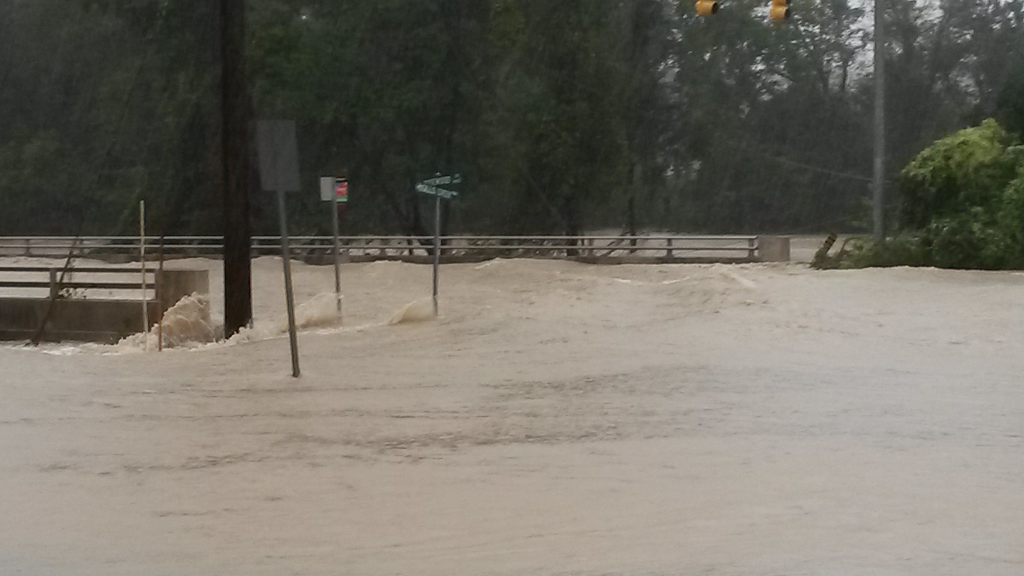
A stalled mid-latitude weather system directed a fire hose of deep tropical moisture across South Carolina over a four-day period (October 2-5) leading to record-breaking rainfall totals. The rainfall lead to extensive flooding across the central and eastern portions of the state. At least 50 state-regulated dams were breached, more than 200 water rescues were performed, and seventeen people lost their lives in the event.
The Weather
The extraordinary rainfall was generated by the movement of very moist air over a stalled frontal boundary near the coast.
The clockwise circulationon around a stalled upper level low over southern Georgia directed a narrow plume of tropical moisture northward and then westward across South Carolina over the course of four days.
The outer circulation of Hurricane Joaquin, situated well off the coast, added additional tropical moisture to the system.
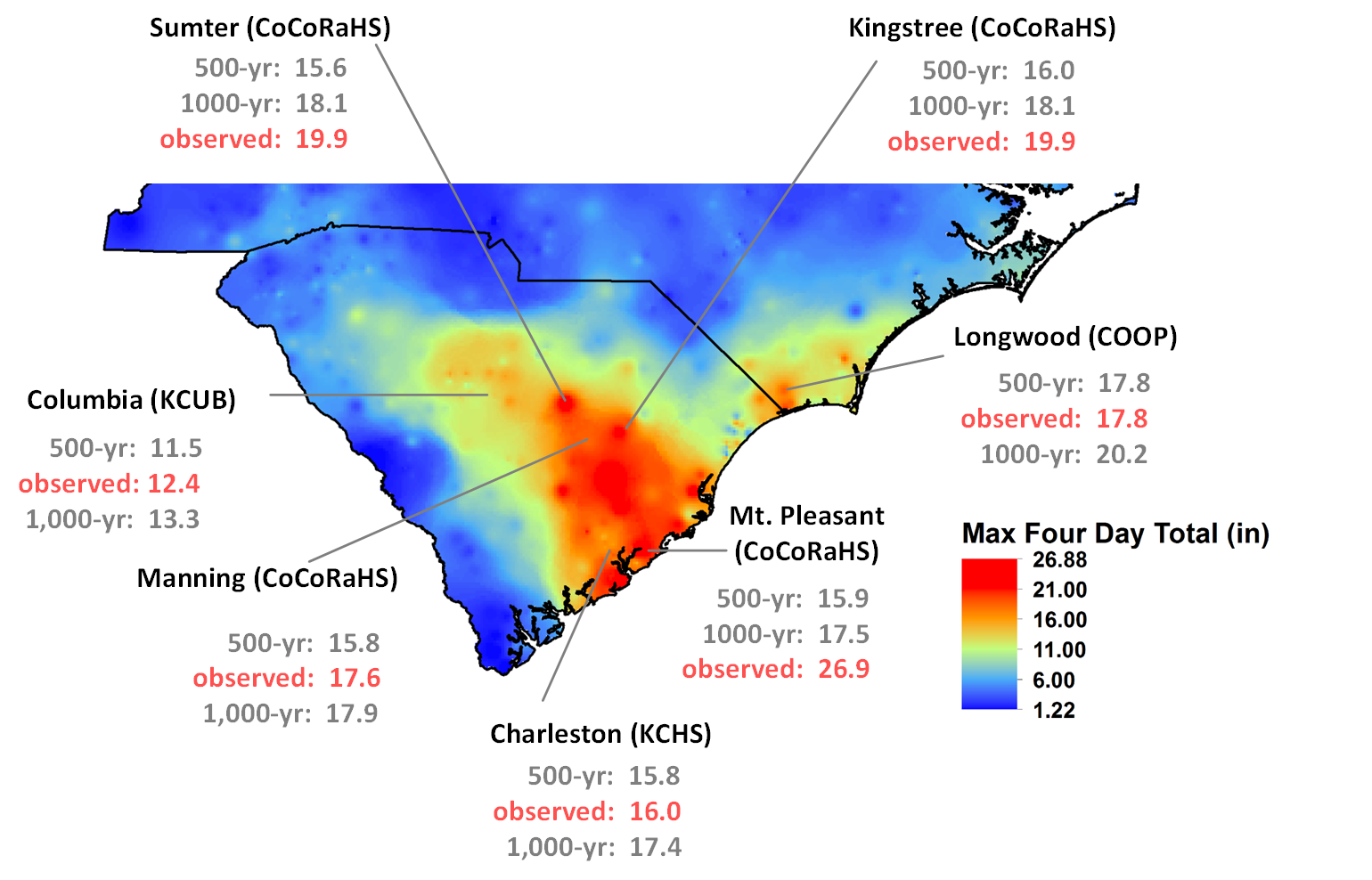
The map below shows the maximum rainfall totals that fell over the 4-day period of this event as well as data from weather stations where 500- and 1000-year recurrence intervals were exceeded. The amount of rain was less than a 1000-year event in some places and greater than that in others. Mt. Pleasant, SC, saw the highest recorded 4-day total (Oct 2-5) at 26.88 inches.
Climate Context
Understanding current climate conditions and previous events that produced similar rainfall amounts places this event in the context of the multiple factors that contribute to the severity of rainfall and flooding events.
Soils were already saturated in many areas prior to the heaviest rainfall on Sunday, October 4, which may have affected patterns of flooding. While the rainfall amounts leading up to October 4 were near-normal in many places, they exceeded 7 inches at several coastal stations north of Charleston, from Georgetown to North Myrtle Beach, and at stations in the greater Columbia area.
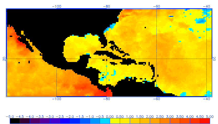
Sea-surface temperatures (SSTs) in the Atlantic were approximately 1.5-2.50°C (3-4.50°F) warmer than average at the beginning of October 2015. This contributed to higher evaporation rates over the Atlantic, feeding more moisture into the weather systems.
Tropical storms often interact with mid-latitude weather features like upper level lows, as happened in this event. In 1990, over 8 inches of rain fell between October 10 and 13 in the Savannah, Edisto, Yadkin–Pee Dee, and Catawba River Basins of North and South Carolina and Georgia. In some isolated spots, rainfall exceeded 12 inches. In the 1990 case, the remnants of Tropical Storm Klaus brought extensive moisture near the SC coast, while Tropical Storm Marco crossed the region from south to north. The influences of these tropical systems was magnified by a stalled cold front, just as it was in October 2015.
Was this a 1000-year flood?
For precipitation, the standard scientific estimates for the probability of rainfall exceeding certain thresholds (also called recurrence intervals) is documented in NOAA’s Atlas 14. The map of rainfall totals above shows observed 4-day total rainfall at selected stations, with reference to recurrence intervals. It is important to remember that the value associated with a 100-year event is the amount of precipitation that, statistically, has a 1% chance of occurring in any given year. A 1000-year event is the precipitation amount that has a 0.1% chance of occurring in any given year. Within the band of heaviest rainfall, several stations exceeded estimates for a 1,000-year event.
The likelihood (or recurrence interval) for a flood is not the same as that for rainfall because factors including the extent and intensity of rainfall and surface conditions (e.g., saturated soils) will influence runoff to streams and rivers. Based on USGS streamgage data, this was not a 1000-year flood. Many gage locations did not break records or even fall within the top 5 flood events. But one also has to consdier that record length for streamgage stations ranges from 5 to 144 years tin SC. This means that in some places there is not a great deal of information, and new information may change the statistics. The USGS has issued a report about this historical event with a table of other major flooding events in South Carolina dating back to 1893.
Hydrological Response
Heavy rains caused severe to extreme flooding across the state although the peak flows at many USGS gages did not break records as rainfall totals did.
The hydrologic response was much longer than the four-day rainfall event. For example, flooding in coastal areas occurred as a result of intense and large amounts of precipitation from October 1-5, and then after the rainfall ended as floodwater flowed downstream. Several stream gages show peak flows through October 11.
The Congaree River peaked early on October 4 as a result of the large rainfall amounts received in the Upstate in the days before the major rainfall event, starting October 3.
Had the upper portion of the Congaree River watershed (e.g., Greenville/Spartanburg area) received precipitation amounts similar to those in the southeastern section of the state there likely would have been a much larger peak discharge, a few days later.
Dams change streamflows and alter the frequency of floods. Comparing information about major floods before and after dam construction provides a broader historical context. For example, the Congaree River peaked at 185,000 cubic feet per second (cfs) on October 4. According to the USGS study, this is the 8th highest peak based on the 123-year record at this gage location. The highest recorded peak (364,000 cfs) occurred in 1908, before the Lake Murray dam was constructed.
Gages where new record peak flows were recorded were mostly in the central to eastern part of SC. This follows from the rainfall amounts, which were substantially greater there.
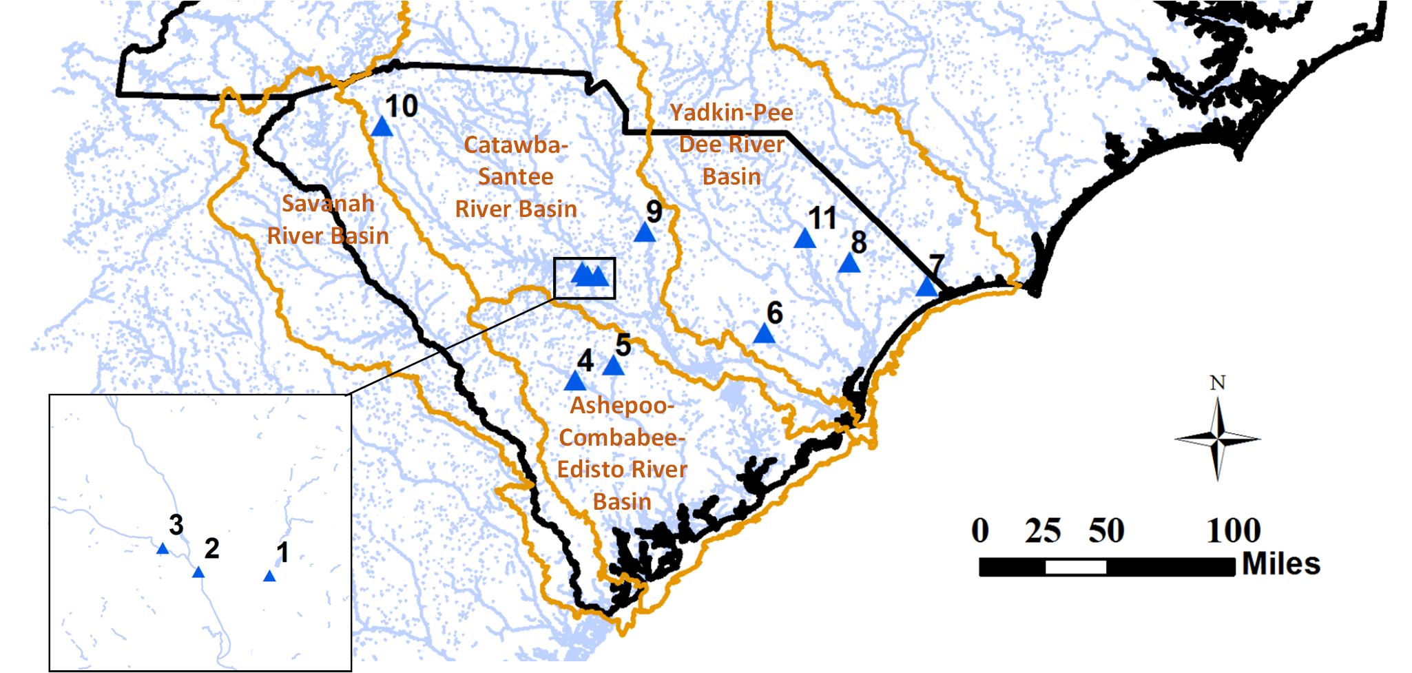
| Gage Number | Gage Location | Oct 2015 Peak (preliminary / cfs) | Peak Day (Oct) | New Record? | Previous or Current Record (cfs and year) | Comments |
|---|---|---|---|---|---|---|
| 1 | Gills Creek at Columbia | >3000 (?) | 4 | Yes (?) | 2,880 (1979) | (?) Gage destroyed |
| 2 | Congaree River near Columbia | 185,000 | 4 | No | 231,000 (1936) | Higher peaks occurred before Lake Murray dam |
| 3 | Saluda River near Columbia | >50,000 (?) | 4 or 5 | Yes (?) | 53,200 (1965) | (?) Gage destroyed; higher peaks before Lake Murray dam |
| 4 | South Fork Edisto River near Denmark | 2,100 | 8 | No | 13,500 (1936) | Many higher peaks |
| 5 | North Fork Edisto near Orangeburg | 8,640 | 5 | No | 9,500 (1945) | -- |
| 6 | Black River at Kingstree | 83,700 | 6 | Yes | 58,000 (1973) | -- |
| 7 | Waccamaw River near Longs | 16,90 | 6 | No | 28,200 (1999) | -- |
| 8 | Little Pee Dee River near Galivants Ferry | 8,230 | 11 | No | 27,600 (1964) | Many higher peaks |
| 9 | Wateree River near Camden | 50,900 | 4 | No | 168,000 (1936) | Many higher peaks; highest pre-date Wateree dam |
| 10 | Saluda River near Greenville | 1,660 | 4 | No | 11,000 (1949) | Many higher peaks |
| 11 | Pee Dee River at Pee Dee | 30,100 | 8 | No | 220,000 (1945) | Many higher peaks; several dams on this river |
Flood Impacts
There are many lessons to be learned about community resilience in the wake of such an extreme event. Particularly important are ways communities can consider rebuilding to avoid similar impacts in the future.
The amount of flood risk South Carolinians face is based on the nature of this event (extreme rainfall on already saturated soils) in combination with their exposure (e.g., proximity to streams and rivers) and the condition of infrastructure, homes, roads, and businesses in the path of the flooding.
The situation in the Gills Creek watershed in Columbia is not straight forward. There were three dam breaches in the early morning of October 4 that cumulatively released a large pulse of water. This, perhaps more than the precipitation itself, was a major cause of the spatial extent and depth of the flooding below Lake Katherine in the Crosshill/Garners Ferry Road area.
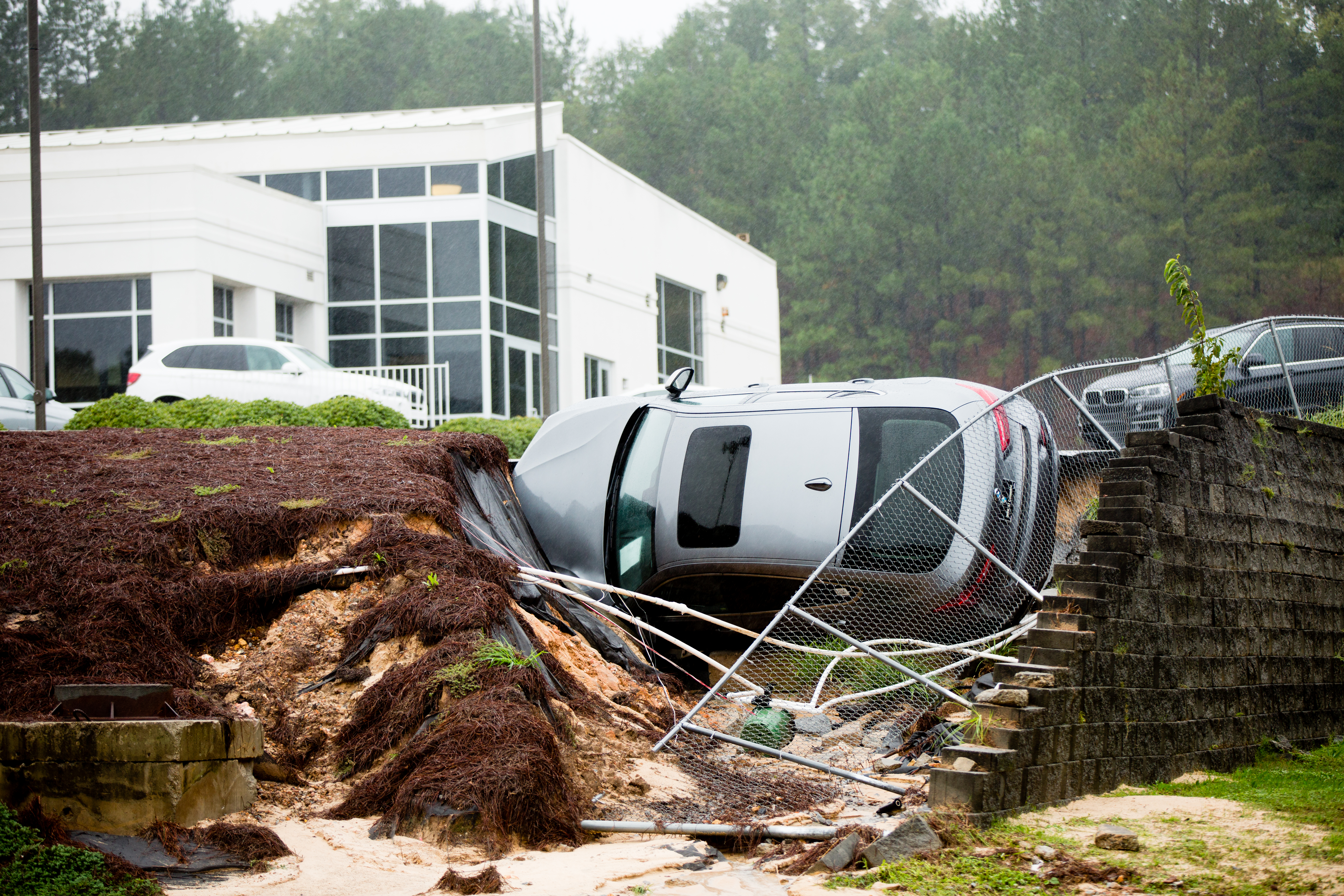
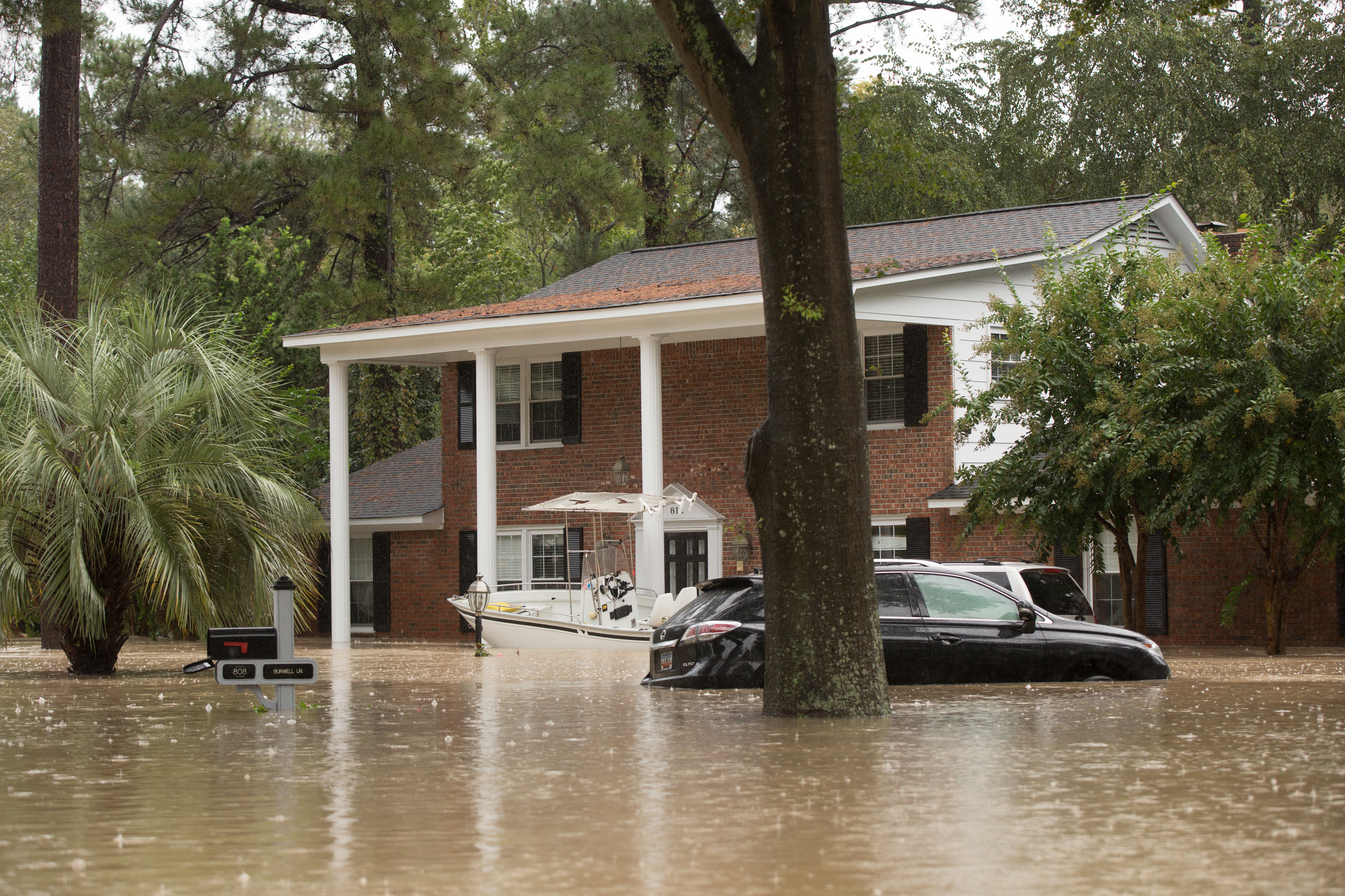
As the region has added population and expanded development, the potential for more and greater impacts from an extreme event has grown. However, these impacts can be reduced or avoided through planning for greater resilience during recovery and future growth.
Flood likelihood estimates are based on statistical averages, not on the number of years between big floods. A so-called 100-year flood has a 1% chance of occurring in any given year. This means that, over the life of a 30-year mortgage, there is a greater than 25% chance that a house in the 100-year floodplain could flood. These estimates of chance are only as good as the available data. As more data are collected on the changing conditions in a river basin (i.e., increased development to create more impervious surface which influences runoff), the estimates may be revised.
Important discussions about how to reduce future impacts are underway. Questions about how to rebuild dams, help families and communities that have fewer resources than others to rebuild, and reduce future flood risk are part of this ongong discussion in the Carolinas.
Additional Resources
The sources below can help you learn more about the 2015 flood.
- SC State Climatology Office
- SC DNR's Journal of South Carolina Flooding 2015
- USGS South Atlantic Water Science Center
- SC Dept of Health & Environmental Control
- SC Coastal Information
- National Weather Service
- South Carolina Public Radio's Narrative Project (see especially the July–December 2016 interviews)